LLM 笔记大杂烩

约 1928 个字 56 行代码 3 张图片预计阅读时间 10 分钟共被读过次

#attention #grouped-query-attention #linear-attention #position-embedding #RMSNorm #RoPE #transformer

施工中……

Attention¶

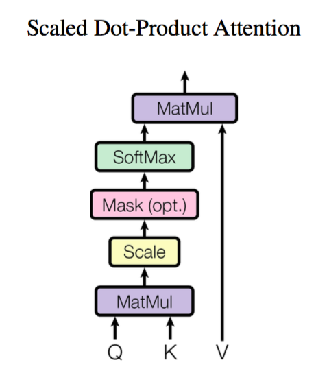
输入序列

\[ X = (x_{0},x_{1},\dots,x_{n-1})^{\top} \in \mathbb{R}^{n\times d_{1}} \]

通过可训练的权重矩阵 \(W^{Q}\in \mathbb{R}^{d_{1}\times d_{k}}\)，得到 queries

\[ Q = XW_{Q} \in \mathbb{R}^{n\times d_{k}} \]

然后对外来的（或者 \(X\) 自己的子序列）

\[ Y = (y_{1},y_{2},\dots,y_{m})\in \mathbb{R}^{m\times d_{2}} \]

通过 \(W^{K}\in \mathbb{R}^{d_{2}\times d_{k}}, W^{V}\in \mathbb{R}^{d_{2}\times d_{v}}\)，有 keys 和 values

\[ \begin{align} K & = YW^{K}\in \mathbb{R}^{m\times d_{k}} \\ V & = YW^{V}\in \mathbb{R}^{m\times d_{v}} \end{align} \]

之后

\[ \text{Attention}(Q,K,V)=\text{softmax}\left( \frac{QK^{\top}}{\sqrt{ d_{k} }} \right)V \in \mathbb{R}^{n\times d_{v}} \]

可以认为是将一个 \(n\times d_{k}\) 的序列 \(Q\) 转化为了新的序列 \(K\in \mathbb{R}^{n\times d_{v}}\)

逐向量版本

\[ \text{Attention}(q_t,K,V) = \sum_{s=1}^m \frac{1}{Z}\exp\left(\frac{\langle q_t, k_s\rangle}{\sqrt{d_k}}\right)v_s \]

Multi-head Attention¶

也就是将 \(Q\)、\(K\)、\(V\) 按照第二个维度拆分后，分别进行计算，然后拼接起来

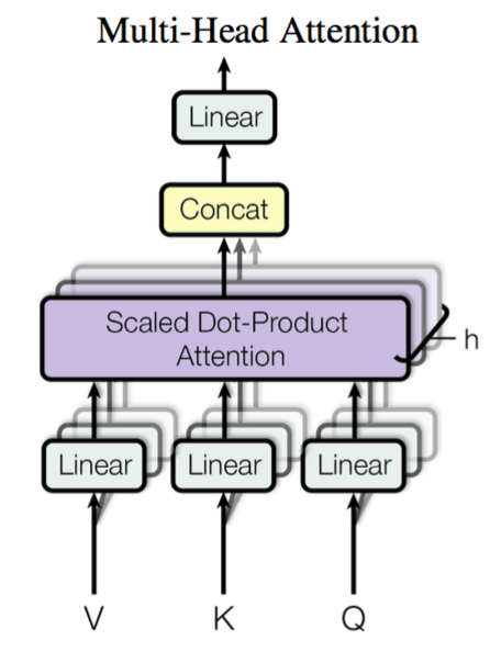
\[ \text{head}_{i} = \text{Attention}(QW_{i}^{Q}, KW_{i}^{K}, VW_{i}^{V}) \]

这里 \(W_{i}^{Q},W_{i}^{K}\in \mathbb{R}^{d_{k}\times \bar{d}_{k}}, W_{i}^{V}\in \mathbb{R}^{d_{v}\times \bar{d}_{v}}\)

之后

\[ \text{MultiHead}(Q,K,V) = \text{concat}(\text{head}_{1},\text{head}_{2},\dots,\text{head}_{h}) \]

Self-Attention¶

只需要将 \(Q\)、\(K\)、\(V\) 都使用一个序列 \(X\) 得到即可

\[ \begin{align} Q_{i} & = XW_{i}^{Q}\in \mathbb{R}^{n\times \bar{d}_{k}} \\ K_{i} & = XW_{i}^{K}\in \mathbb{R}^{n\times \bar{d}_{k}} \\ V_{i} & = XW_{i}^{V}\in \mathbb{R}^{n\times \bar{d}_{v}} \end{align} \]

之后得到多头注意力

\[ \text{head}_{i} = \text{Attention}(Q_{i},K_{i},V_{i}) \in \mathbb{R}^{n\times \bar{d}_{v}} \]

拼接后得到

\[ \text{MutilHead}(Q,K,V) = \text{concat}(\text{head}_{1}, \text{head}_{2},\dots,\text{head}_{n}) \in \mathbb{R}^{n\times d_{v}} \]

可以取 \(d_{v}\) 和 \(X\) 序列的每一个向量维度（即 \(X\) 的第二维度）相同

Linear Attention¶

在最原始的 attention 中，计算复杂度是 \(O(n^{2})\)，主要是由 softmax 引起的，更一般的，attention 公式可以写作

\[ \text{Attention}(Q,K,V) = \frac{\sum_{j=1}^{n}\text{sim}(q_{i},k_{j})v_{j}}{\sum_{j=1}^{n} \text{sim}(q_{i},k_{j})} \]

其中相似度函数 \(\text{sim}\) 需要满足非负性，也因此无法简单的去除原式中的 softmax 以加快矩阵运算 \((n\times d_{k})\times(d_{k}\times m)\times(m\times d_{v})\)

核函数形式¶

将 \(q_{i},k_{j}\) 用核函数映射到非负区域上，从而保证非负，即

\[ \text{sim}(q_{i},k_{j}) = \phi(q_{i})^{\top}\psi(k_{j}) \]

利用 Softmax 特殊性质¶

只要先对 \(Q\) 的 \(d\) 那一维和 \(K\) 的 \(n\) 那一维进行 softmax，那么得到的结果自动满足归一化条件：

\[ \text{LinearAttention} = \text{softmax}_{2}(Q)\cdot \text{softmax}_{1}(K)^{\top} V \]

Grouped Query Attention¶

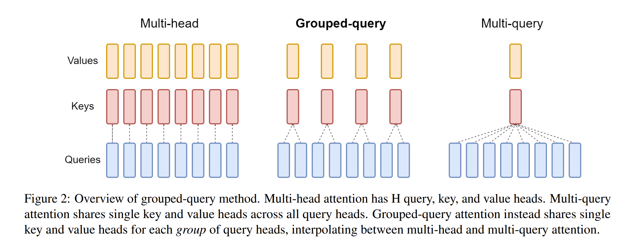
Queries heads 被分为了若干个组，每个组内共享同一个 key head 和 value head。划分组的方法：

Grouping queries based on similarity: computing a similarity metric between queries and then assigning them to groups accordingly.
Dividing query heads into groups: query heads are divided into groups, each of which shares a single key head and value head.
Using an intermediate number of key-value heads
Repeating key-value pairs for computational efficiency: key-value pairs are repeated to optimize performance while maintaining quality

优点：

Interpolation 减少了 MHA 和 MQA 中 quality degradation、training instability 等问题
Efficiency 通过选择恰当的 key-value heads 组数，提高效率的同时保持了质量
Trade-off 在 MHA 和 MQA 中保证了质量

代码可参考：GitHub - fkodom/grouped-query-attention-pytorch: (Unofficial) PyTorch implementation of grouped-query attention (GQA) from "GQA: Training Generalized Multi-Query Transformer Models from Multi-Head Checkpoints" (https://arxiv.org/pdf/2305.13245.pdf)

Position Embedding¶

为了表征 token 的相对位置，可以引入位置编码，否则 transformer 将无法辨认词语间的先后关系。

Sinusoidal¶

Google 的原始论文中给出的编码为

\[ \begin{cases} \text{PE}_{2i}(p) = \sin\left( \frac{p}{10000^{2i/d_{P}}} \right) \\ \text{PE}_{2i+1}(p) = \cos \left( \frac{p}{10000^{2i/d_{P}}} \right) \\ \end{cases} \]

其中 \(P\) 为序列总长度。之所以使用这个表达式，是为了便于表征相对位置，因为有

\[ \begin{align} \sin(\alpha+\beta) & =\sin\alpha \cos \beta + \sin \beta \cos \alpha \\ \cos(\alpha+\beta) & =\cos \alpha \cos \beta-\sin \alpha \sin \beta \end{align} \]

即第 \(p+k\) 位的表征可以由第 \(p\) 位的表征加上 \(k\) 位的偏移得到

RoPE¶

为了实现使用绝对位置编码的方式实现相对位置编码，经过推导（见 reference 3），得到对二维向量 \(\vec{q}\)，在 \(m\) 处的位置编码为

\[ f(\vec{q},m) = R_{f}(\vec{q},m)e^{i\Theta_{f}(\vec{q},m)} = \lVert \vec{q} \rVert e^{i(\Theta(\vec{q}) + m\theta )} = \vec{q}e^{im\theta } = \begin{pmatrix} \cos m\theta & -\sin m\theta \\ \sin m\theta & \cos m\theta \end{pmatrix}\begin{pmatrix} q_{0} \\ q_{1} \end{pmatrix} \]

即对应向量 \(\vec{q}\) 旋转 \(m\theta\) 的角度。对于任意偶数维的 RoPE，可表示为二维情形的拼接，即

\[ \scriptsize{\underbrace{\begin{pmatrix} \cos m\theta_0 & -\sin m\theta_0 & 0 & 0 & \cdots & 0 & 0 \\ \sin m\theta_0 & \cos m\theta_0 & 0 & 0 & \cdots & 0 & 0 \\ 0 & 0 & \cos m\theta_1 & -\sin m\theta_1 & \cdots & 0 & 0 \\ 0 & 0 & \sin m\theta_1 & \cos m\theta_1 & \cdots & 0 & 0 \\ \vdots & \vdots & \vdots & \vdots & \ddots & \vdots & \vdots \\ 0 & 0 & 0 & 0 & \cdots & \cos m\theta_{d/2-1} & -\sin m\theta_{d/2-1} \\ 0 & 0 & 0 & 0 & \cdots & \sin m\theta_{d/2-1} & \cos m\theta_{d/2-1} \\ \end{pmatrix}}_{{\mathcal{R}}_m} \begin{pmatrix}q_0 \\ q_1 \\ q_2 \\ q_3 \\ \vdots \\ q_{d-2} \\ q_{d-1}\end{pmatrix}} \]

对于 query \(q\) 和 key \(k\)，分别乘上旋转矩阵 \(\mathcal{R}_{m}\) 和 \(\mathcal{R}_{n}\) 就相当于：

\[ (\mathcal{R}_{m}q)^{\top}(\mathcal{R}_{n}k) = q^{\top}(\mathcal{R}_{m}^{\top}\mathcal{R}_{n})k = q^{\top}\mathcal{R}_{n-m}k \]

又由于 \(\mathcal{R}_{m}\) 的稀疏性，不使用矩阵乘法，而是用

\[ \begin{pmatrix}q_0 \\ q_1 \\ q_2 \\ q_3 \\ \vdots \\ q_{d-2} \\ q_{d-1} \end{pmatrix}\otimes\begin{pmatrix}\cos m\theta_0 \\ \cos m\theta_0 \\ \cos m\theta_1 \\ \cos m\theta_1 \\ \vdots \\ \cos m\theta_{d/2-1} \\ \cos m\theta_{d/2-1} \end{pmatrix} + \begin{pmatrix}-q_1 \\ q_0 \\ -q_3 \\ q_2 \\ \vdots \\ -q_{d-1} \\ q_{d-2} \end{pmatrix}\otimes\begin{pmatrix}\sin m\theta_0 \\ \sin m\theta_0 \\ \sin m\theta_1 \\ \sin m\theta_1 \\ \vdots \\ \sin m\theta_{d/2-1} \\ \sin m\theta_{d/2-1} \end{pmatrix} \]

可以看出 RoPE 是“乘性”的位置编码，而 sinusoidal 是“加性”的。

RoPE 还是目前唯一一种可以用于 Linear Attention 的相对位置编码。

二维情形¶

上面是在 NLP 中的应用，如果想推广到图像等二维数据中，可以推广为

\[ \mathcal{R}_{x,y} = \begin{pmatrix} \cos x\theta & -\sin x\theta & 0 & 0 \\ \sin x\theta & \cos x\theta & 0 & 0 \\ 0 & 0 & \cos y\theta & -\sin y\theta \\ 0 & 0 & \sin y\theta & \cos y\theta \end{pmatrix} \]

即将输入向量分为两半，一半使用一维的 x-RoPE，一半使用一维的 y-RoPE。并且由于这个矩阵是正交的，在给定 \(\mathcal{R}_{x,y}\) 后可以反解出 \(x\) 和 \(y\)。

代码实现¶

Python

# 照搬 llama 的源码，写了点注释
import torch

def apply_rotary_emb(
    xq: torch.Tensor,
    xk: torch.Tensor,
    freqs_cis: torch.Tensor,
) -> Tuple[torch.Tensor, torch.Tensor]:
    # *xq.shape[:-1]: 将第 0 维到倒数第 2 维保留，最后一维两两配对，并视作复数
    xq_ = torch.view_as_complex(xq.float().reshape(*xq.shape[:-1], -1, 2))
    xk_ = torch.view_as_complex(xk.float().reshape(*xk.shape[:-1], -1, 2))
    freqs_cis = reshape_for_broadcast(freqs_cis, xq_) # 便于广播的辅助han
    xq_out = torch.view_as_real(xq_ * freqs_cis).flatten(3) # 元素间相乘，然后从第三维（head_dim 那维）开始拉平，即将之前的两两配对视为复数展开为实数
    xk_out = torch.view_as_real(xk_ * freqs_cis).flatten(3)
    return xq_out.type_as(xq), xk_out.type_as(xk)

而 freqs_cis 按照论文的实现为：

freqs_cis 实现

Python

import torch
def precompute_freqs_cis(dim: int, end: int, theta: float = 10000.0):
    """
    Precompute the frequency tensor for complex exponentials (cis) with given dimensions.

    This function calculates a frequency tensor with complex exponentials using the given dimension 'dim'
    and the end index 'end'. The 'theta' parameter scales the frequencies.
    The returned tensor contains complex values in complex64 data type.

    Args:
        dim (int): Dimension of the frequency tensor.
        end (int): End index for precomputing frequencies.
        theta (float, optional): Scaling factor for frequency computation. Defaults to 10000.0 （论文中的默认值）.

    Returns:
        torch.Tensor: Precomputed frequency tensor with complex exponentials.
    """
    # Calculate the frequency scaling factors for the dimension.
    freqs = 1.0 / (theta ** (torch.arange(0, dim, 2)[: (dim // 2)].float() / dim))
    # Create a tensor of integers from 0 to 'end - 1' on the same device as 'freqs'.
    t = torch.arange(end, device=freqs.device)  # type: ignore
    # Compute the outer product of 't' and 'freqs' to get the frequency matrix.
    freqs = torch.outer(t, freqs).float()  # type: ignore
    # Convert the frequency matrix to a complex tensor using polar coordinates.
    freqs_cis = torch.polar(torch.ones_like(freqs), freqs)  # complex64, 用复数表示
    # Return the complex frequency tensor.
    return freqs_cis

Normalization¶

RMSNorm¶

相比 LayerNorm，RMSNorm 没有减去均值的步骤，而是直接除以均方根：

\[ \begin{align} \text{RMS}(x) & = \sqrt{ \frac{1}{d}\sum_{i=1}^{d} x_{i}^{2} + \epsilon } \\ \hat{x} & =\frac{x}{\text{RMS}(x)} \\ y & = \gamma \cdot \hat{x} \end{align} \]

其中 \(\gamma\) 为超参数（也可以被训练）；\(\epsilon\) 是为了防止 \(\text{RMS}(x)=0\)

用 RMSNorm 替代 LayerNorm 的可能原因为：

计算效率更高
超参数更少
研究表明，减去均值（均匀化）对模型性能影响有限，而缩放操作（rescaling）影响更大
硬件友好：无须计算均值，便于并行化

代码实现

Python

import torch.nn as nn
import torch

class RMSNorm(nn.Module):
    def __init__(self, dim, eps=1e-5):
        super().__init__()
        self.gamma = nn.Parameter(torch.ones(dim))
        self.eps = eps

    def forward(self, x: torch.Tensor):
        rms = torch.rsqrt(x.pow(2).mean(-1, keepdim=True).sqrt() + self.eps)
        x_hat = x / rms
        out = self.gamma * x_hat
        return out

LLM 笔记大杂烩

Attention¶

Multi-head Attention¶

Self-Attention¶

Linear Attention¶

核函数形式¶

利用 Softmax 特殊性质¶

Grouped Query Attention¶

Position Embedding¶

Sinusoidal¶

RoPE¶

二维情形¶

代码实现¶

Normalization¶

RMSNorm¶

Reference¶